You (Probably) Shouldn't use a Lookup Table
I have been working on another post recently, also related to division, but I wanted to address
a comment I got from several people on the previous division article. This comment invariably
follows a lot of articles on using math to do things with chars and shorts. It is: "why
are you doing all of this when you can just use a lookup table?"
Even worse, a stubborn and clever commenter may show you a benchmark where your carefully-crafted algorithm performs worse than their hamfisted lookup table. Surely you have made a mistake and you should just use a lookup table. Just look at the benchmark!
When you have only 8 or 16 bits of arguments, it is tempting to precompute all of the answers and throw them in a lookup table. After all, a table of 256 8-bit numbers is only 256 bytes, and even 65536 16-bit numbers is well under a megabyte. Both are a rounding error compared to the memory and code footprints of software today. A lookup table is really easy to generate, and it's just one memory access to find the answer, right?
The correct response to the lookup table question is the following: If you care about performance, you should almost never use a lookup table algorithm, despite what a microbenchmark might say.
CPU Cache Hierarchy
Unfortunately, with many performance-related topics, the devil is in the details. The pertinent detail, for lookup tables, is hidden in the "one memory access." How long does that memory access take?
It turns out that on a modern machine, it depends a lot on a lot of things, but it is usually a lot longer than our mental models predict. Let's take the example of a common CPU: an Intel Skylake server CPU. It turns out that on a Skylake CPU, that memory access takes somewhere between 4 and 250 CPU cycles! Most other modern CPUs have a similar latency range.
The variance in access latency is driven by the cache hierarchy of the CPU:
- Each core has 64 kB of dedicated L1 cache, split equally between code and data (32k for each)
- Each core has 1 MB of dedicated L2 cache
- A CPU has 1.375 MB of shared L3 cache per core (up to about 40 MB for a 28-core CPU)
These caches have the following access times:
- 4-5 cycle access latency for L1 data cache
- 14 cycle access time for L2 cache
- 50-70 cycle access time for L3 cache
Main memory has an access latency of about 50-70 ns (100-210 cycles for a Skylake server chip) on top of the L3 access time. Dual-socket machines, as are used in cloud computing environments, have an additional ~10% memory access time penalty to keep the caches coherent between the two sockets.
Here, we are disregarding throughput, but suffice it to say that L1 and L2 caches have nearly unlimited throughput, the L3 cache has enough to do most things you would want to do with lookup tables, and main memory never has enough.
A Brief Introduction to Caches
Caches are designed to help with common memory access patterns, generally meaning linear scans
of arrays, while also being constrained by hardware engineering constraints. To that end, caches
don't operate on arbitrary-sized variables, only 64-byte cache lines. When a memory access
occurs, a small memory access for a single char is translated into a memory access for a 64-byte
cache line. Then, the L1 cache allows the CPU to do operations smaller than 64 bytes.
A memory access to a cache line that is in a cache is called a cache hit, and an access to a cache line that must be fetched from memory (or from another cache) is a cache miss. Caches can only hold so many cache lines, so once a line has expired from the cache (which happens when it has not been hit recently), it is evicted, at which point, the next access to that cache line will be a cache miss.
To make the hardware smaller, caches are also generally split up into sets. Each memory address is associated with only one set in a cache, so instead of looking through the entire cache to see if you have a cache hit, you only have to look within a set. The sets tend to be small: the L1 caches on a Skylake CPU have 8 slots (or "ways"). Thus, the Skylake L1 cache is an "8-way set associative cache" because it has 8 ways. A cache that has only one way is called "direct mapped" and a cache without set associativity (where a cache line can reside anywhere in the cache) is called "fully associative." Fully associative caches take a lot of power and area, and direct-mapped caches take the least. The L2 cache on a Skylake is 16-way set associative, and the L3 cache is 11-way set associative.
The set size of a cache influences how long a cache line is likely to stay in the cache: the more associativity the cache has (the more ways there are), the longer it will take for a cache line to be evicted. For example, a fully associative cache that holds 100 cache lines will only evict a line after 100 memory accesses. On the other hand, a direct mapped cache can evict a cache line on the next memory access, if that access happens to map to the same set as the previous access.
In theory, if you are performing a linear scan of a large array, you are going to scan through the entire line, so the cache doesn't waste bandwidth operating this way. If you aren't scanning an array, you may be accessing a local variable, and if you are, you will likely access another local variable nearby, within the same cache line. In turn, compilers and performance engineers take cache locality into account, improving the effectiveness of the cache.
In addition, the caches have prefetching logic which can predict when a memory access is going
to occur, and fetch the appropriate cache line. Thus, if you are doing a linear scan, the
prefetch logic can help you avoid taking any cache misses at all! You can also influence the
prefetch logic on an x86 core with instructions like PREFETCHT0, but these are only requests,
not direct instructions.
Processors can have different sized cache lines, but many CPUs (including all x86 CPUs) use 64 bytes. That is also the same size as a DDR4 transfer, so it is convenient for memory systems to work with 64 byte units and nothing smaller.
Lookup Tables and Caches
When comparing a lookup table to the alternative, it is important to think about where the lookup table needs to be situated in order to have a speed advantage. In most cases where a lookup table will be worth using, you will want the lookup table to have an advantage if it is in the L3 cache or above and you want the function to be called enough that the table stays there. To take an absurd example, consider a function that outputs the result of the subset-sum problem on a particular set for a given target. It is much faster to precompute all of the subset-sum results and then put them in a lookup table than to try to compute each solution on the fly.
Simulating Lookup Tables with a Cache Hierarchy
To prove my point, I made a simple simulation. The simulation tracks data accesses of a single core of a program, and tracks the population of the cache lines. We are assuming that the memory footprint of the program is 1 GB in total, and that it accesses memory addresses in an exponentially distributed way when it is not using the lookup table.
As a simplifying assumption, we are ignoring code access and assuming that there are 0 bytes of code outside the L1 instruction cache. We also assume that the L3 cache is strictly partitioned so that the one core gets 1.375 MB of it, and we are simulating only one core (assuming that other cores are doing other work). Finally, we are assuming that the cache follows an LRU eviction policy, and will always evict the least recently used cache line in a set. We are also assuming the following latencies for a lookup:
- 4 cycles for L1 cache
- 14 cycles for L2 cache
- 50 cycles for L3 cache
- 200 cycles for main memory
The simulator will let us simulate several different types of access patterns, but the two access patterns we will use are the following:
- Even distribution of intervening memory accesses - this is an academic exercise that helps us understand the impact of caching on performance of lookup tables.
- Bursty distribution of intervening memory accesses, modeled with an exponential distribution - this is a lot closer to how a real program will look: short bursts of function calls will be interspersed with longer gaps where no use of the lookup table occurs.
For both categories, we will be simulating points in the range between 0 and 500 expected intervening memory accesses between lookup table accesses. Here are a few example guidelines to think about, although the actual meaning of "intervening memory accesses" is program-dependent:
- 0-5 intervening memory accesses: this is basically a microbenchmark. Likely all you are doing is reading values, using the lookup table, and writing values back.
- ~20 intervening memory accesses: the lookup table function is one of the core functions in a program.
- ~100 intervening memory accesses: the lookup table function is one of the major functions used, but not at the top of the CPU profile.
- ~500 intervening memory accesses: the lookup table function is warm, but not particularly hot.
Distilling down to a few regimes:
- 0-10 - microbenchmarks and benchmarks
- 10-100 - hot functions, usually the region of interest for optimization
- 100-500 - warm functions that may or may not be of interest
Example 1: A 256-byte Lookup Table
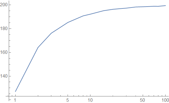
Let's take the example of a small lookup table, a 256-byte table, and let's assume that it is accessed uniformly randomly. The table is 4 cache lines long. Here's the access latency in cycles that we get from our simulation, plotted against the period of access on a log scale (1 = every memory access goes to the lookup table, and 100 = 1% of accesses go to the lookup table):
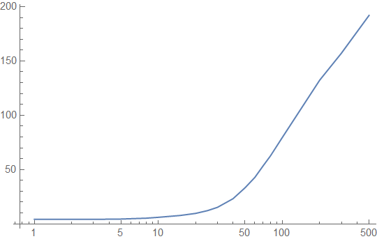
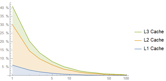
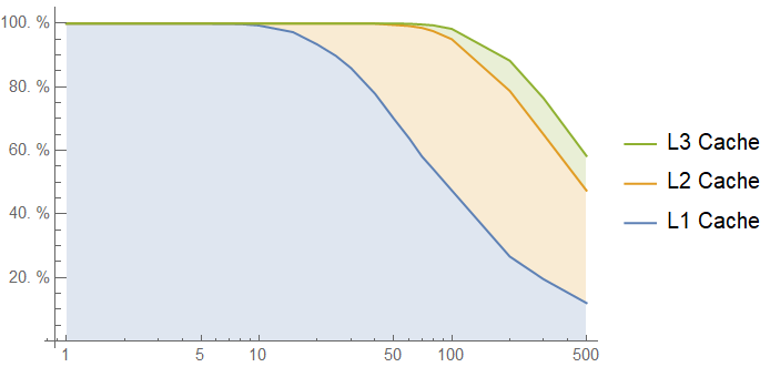
Here is the cache hit rate for accesses to our lookup table against log-scaled number of intervening memory accesses:
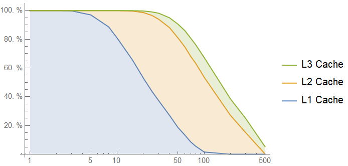
If we are in the "extremely hot function" range, with less than 20 intervening memory accesses, the lookup table function looks great. If not, it doesn't look so great.
It seems to defy expectations that such a small lookup table would be getting evicted from a cache so quickly. However, let's think about the access pattern for the lookup table: on each access, we are only touching one of its cache lines. Since there are 4 cache lines in the lookup table, each cache line effectively sees 4 times as many intervening accesses as the entire lookup table sees. This means that we should actually expect the lookup table to be much further down the cache hierarchy than we would think given its small size.
This is not analogous to the case of 256 bytes of code or 256 bytes of local variables: we expect to touch every cache line in the code and every cache line of local variables each time the function is called. We could attempt to rectify this by adding prefetching instructions for all of the cache lines, but this will not be a panacea either, and most importantly, it will hurt our latency floor when the function is called very often.
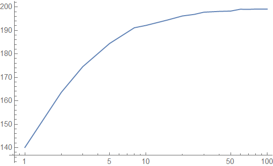
Here are our performance graphs on bursty (non-uniform) accesses to the lookup table:
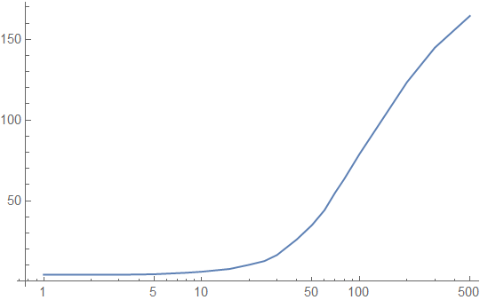
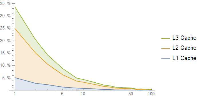
The ceiling of the chart here is far better, around 160 cycle latency on average instead of 200 cycle latency, and as we can see in the caching plot below, the cache hierarchy helps a lot with occasional burst accesses to the lookup table:
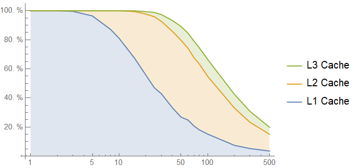
Even with an average of 500 memory accesses between each lookup table call, 30% of accesses to the lookup table are cached! However, in the useful window between 10 and 100 intervening memory accesses, we get very similar performance to the uniform access simulations. This should not be surprising: most of those accesses are already coming out of caches, and even though we shift more of them to the L1 cache, there are also longer gaps between bursts during which the lookup table is evicted down the cache hierarchy.
Example 2: A 65536-byte Lookup Table
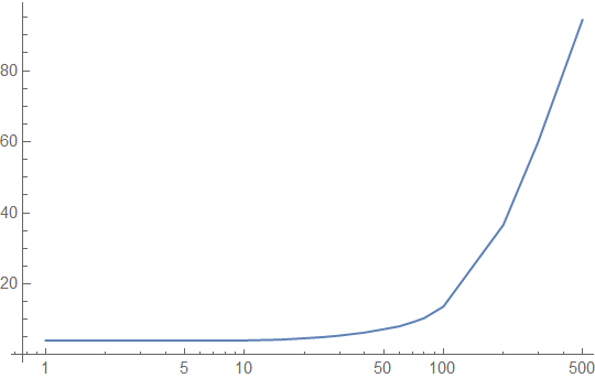
Let's take the example of a large lookup table corresponding to 16 input bits. Again, we will assume that it is accessed uniformly randomly. Our latency profile (again, in clock cycles) looks like:
That's not so good - it looks like we are almost working out of main memory to start! Note that this graph cuts off at 100 intervening accesses, because after that point, the average latency is almost equal to the memory latency. Here is the cache hit rate, confirming our suspicions:
This is an extreme example, but the conclusion we get here is pretty stark: if you want to use a lookup table of several KB, expect it to take a long time. Each cache line of this lookup table sees 1024 times more intervening memory accesses than the entire table sees!
For a bursty access pattern, we actually see worse performance results than our uniform access pattern:
You need a very long burst to cache the entire lookup table, and each cache line of your table is an antagonist for the other cache lines of the table. We get the following cache hit rates from the bursty access pattern:
Example 3: A 64-byte Lookup Table
Finally, let's look at a lookup table that is a single cache line, and see how well it performs. You can't look up many values in this table, but it illustrates how the effects of the cache hierarchy are amplified by the size of the lookup table. Here's how the 64-byte lookup table looks with a realistic, bursty access pattern:
Note that the latency graph tops out at around 90 cycles, unlike previous charts, and 60% of accesses are cached. The "critical region" between 10 and 100 intervening accesses is served mostly from the L1 cache, and cached 100% of the time.
This is good. A single cache line lookup table has great performance for a warm function. If the function is not warm, we don't care much either, since it's not a significant performance driver of the overall system. For caching purposes, a lookup table that fits in a single cache line behaves like a constant or a local variable: It is going to be accessed on every invocation of the function, so it is going to be in the cache if the function was called recently, and its performance is not data-dependent.
Bringing it All Together
A comparison of the performance of lookup tables in all of our simulations is here, alongside a simulation for a 2 kB lookup table:
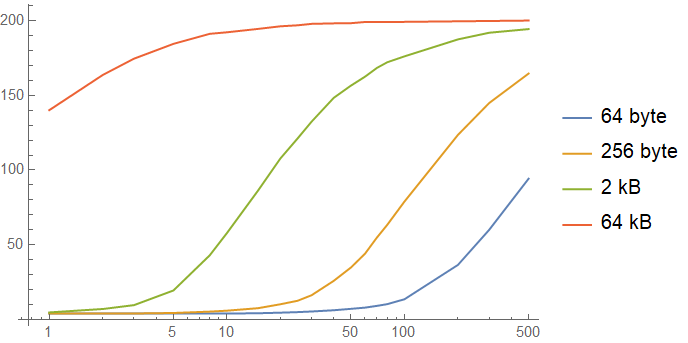
These siumulations show us the problem of lookup tables and microbenchmarks: the cache hierarchy completely destroys the results of the benchmark by operating on the far left side of the graph. Most bits of code tend to perform slightly better in microbenchmarks than in situ thanks to the cache hierarchy, but lookup tables get an extreme version of this benefit. Once your lookup table gets evicted down the cache hierarchy, it starts to slow down significantly.
Unfortunately, the range between "10" and "100" on this graph is the critical zone for performance- sensitive functions, and that is the region where even small lookup tables start to get slow and start to see a lot of variance in their performance. This is when the caching architecture of modern CPUs tends to stop favoring you.
Non-uniform Access Patterns
Up to this point, we have been assuming a uniform random access to the lookup table. Sometimes this is not true. If we have nonuniform access patterns, the commonly-accessed parts of the lookup table are more likely to be closer to the core, but the uncommonly accessed parts are likely to be farther.
To look at this case, I simulated access to the lookup table using an exponentially distributed pattern to simulate a non-uniform access pattern. In one simulation, 63% of acceses (1 standard deviation) go to the first cache line. In the next simulation, 95% of accesses (2 standard deviations) go to the first cache line. The results of the simulation, with the 64B table and a uniform access pattern for comparison are below:
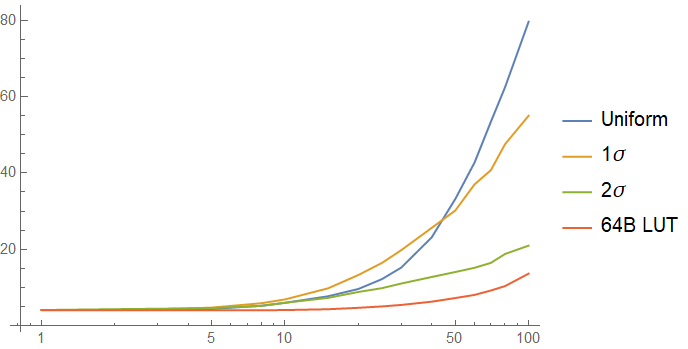
The one sigma case may have worse performance than the uniform case! The cache misses incurred on the other cache lines of the table are expensive, and more than make up for the performance gain you get from one cache line being a lot hotter than in the uniform case. As the function gets colder, non-uniform access to the lookup table starts to help a lot - I cut this graph off at 100 intervening accesses to show the interesting region better, but the trends you see at 100 continue.
As expected, the two sigma case performs very similarly to the case of a lookup table that is a single cache line in the tail, but the performance of the 256 byte table whose first 64 bytes see 95% of accesses is similar to that of the uniformly accessed table on the left side of the graph: the rare cache misses on other cache lines hurt a lot.
What about the cost of code?
An easy argument against what we have said so far is: "Fine, the lookup table is not very cache efficient, but neither is the extra kilobyte of code that you use to avoid a lookup table! That has to be fetched from memory too!"
It's true that the code does have to be fetched from memory, and a larger code footprint increases the chance of an instruction cache miss. However, there are three significant mitigating factors in terms of the cost of cache misses on code:
- The "heat" of code tends to be much more unevenly distributed than data
- Code tends to be easy to prefetch unless it is branchy
- Code is usually touched on every invocation of a function unless it branches
Combining all of these factors gives you a low instruction cache miss rate for most programs: The L1 instruction cache can consume 64 bytes per cycle, but the instruction fetch unit accepts 16 bytes per cycle. As a result, code can actually be perfectly prefetched through a few branches (not including loops, which are already in the cache), and adding a branch can actually be more costly than adding bytes. Every byte being touched on every invocation helps a lot, too. Finally, the fact that code tends to have a few hot parts and a large cold region indicates is a double-edged sword: raising the hot path over a certain threshold can have a high cost, but until the hot path is a certain size, you can add code without too much of a caching cost.
This is why specific-length-optimized SIMD algorithms for the mem* functions and a lot of other
similar tricks work well: up to a certain program size, the extra code actually doesn't cost much,
especially when that code is either looping or going in a straight line. Of course, there are limits.
When to use Lookup Tables
Lookup table algorithms in software engineering projects are justified in four situations:
- where the lookup table is one cache line or less
- where a full-system benchmark shows that the lookup table algorithm is faster
- where you don't care about performance and it is the easiest algorithm to understand
- where you have complete control of the cache hierarchy (eg on a DSP, not a server CPU)
We have covered the first case, so I won't go into it here.
The second case is straightforward, but easy to mess up. Lookup tables are liars, and can't be trusted unless you have a significant quantity of code around them. If a full-system benchmark shows that you should use a lookup table algorithm, then you should use it. A microbenchmark or a benchmark of a small part of the system does not apply! It will usually be the case that a full-system benchmark suggests using a lookup table when your function is called often enough that the table stays warm, and a smaller table will work out more often than a larger one.
The third case is the easiest to consider. Write something readable. If the lookup table is the most readable thing to do, do it, but please make sure you describe how the table was generated.
The fourth case does not apply to general-purpose CPUs. DSPs and special-purpose processors often have
scratchpads instead of (or in addition to) caches, so you actually can guarantee that your lookup table
will be quickly accessible as long as you are willing to spend some of your limited scratchpad RAM on
the table. GPUs have a region of "constant" memory which can be accessed quickly and can be used
for lookup tables. If you are working with a microcontroller that has only RAM and flash, there is
no cache hierarchy, so you have complete control. These are all places where lookup tables can work
well. While modern desktop and server CPUs do allow you to perform some limited cache manipulation
and provide hints to the prefetch unit, there is currently no way to force a cache line to stay in a
cache. The PREFETCH* instructions are just hints!
Conclusions
Lookup tables have a time and a place, but it's not all the time and it's definitely not everywhere. In performance software engineering, arguments in favor of lookup tables generally have to be very subtle and well-thought-out if you want to make sure that they are actually correct. Even a small lookup table can be a lot worse than the alternatives unless it is used extremely frequently, and a large lookup table should almost never be used.
Further, unlike with other algorithms, a microbenchmark is not a representative measure of performance for a lookup table algorithm unless it is all you are doing, since the distorting effects of the cache hierarchy are magnified for lookup table algorithms. Lookup tables also introduce data dependence on performance, so they are not suitable for algorithms where you need determinism, like in cryptography.
When we think about performance, it is important to make sure that we consider the full picture. Algorithms that are so dependent on their use characteristics and the structure of the hardware can make it very hard to do that. Memory speed hasn't kept up with the speed of CPUs, and so a lot of silicon on a modern processor is made to cope with that fact. As a result, many other algorithms are built around the idea of reducing reliance on memory speed. Lookup tables depend on it to a fault.