Racing the Hardware: 8-bit Division
Occasionally, I like to peruse uops.info. It is a great resource for micro-optimization:
benchmark every x86 instruction on every architecture, and compile the results. Every time I look at this table,
there is one thing that sticks out to me: the DIV instruction. On a Coffee Lake CPU, an 8-bit DIV takes
a long time: 25 cycles. Cannon Lake and Ice Lake do a lot better, and so does AMD. We know that divider
architecture is different between architectures, and aggregating all of the performance numbers for an
8-bit DIV, we see:
| Microarchitecture | Micro-Ops | Latency (Cycles) | Reciprocal Throughput (Cycles) |
|---|---|---|---|
| Haswell/Broadwell | 9 | 21-24 | 9 |
| Skylake/Coffee Lake | 10 | 25 | 6 |
| Cannon Lake/Rocket Lake/Tiger Lake/Ice Lake | 4 | 15 | 6 |
| Alder Lake-P | 4 | 17 | 6 |
| Alder Lake-E | 1 | 9-12 | 5 |
| Zen+ | 1 | 9-12 | 13 |
| Zen 2 | 1 | 9-12 | 13 |
| Zen 3 | 2 | 10 | 4 |
Intel, for Cannon Lake, improved DIV performance significantly. AMD also improved performance between Zen 2 and Zen 3, but was doing a lot better than Intel to begin with. We know that most of these processors have hardware dividers, but it seems like there should be a lot of room to go faster here, especially given the performance gap between Skylake and Cannon Lake.
Before you check out thinking that we can't even get close to the performance of the hardware accelerated division units in modern CPUs, take a look at the benchmark results (lower is better on both graphs):
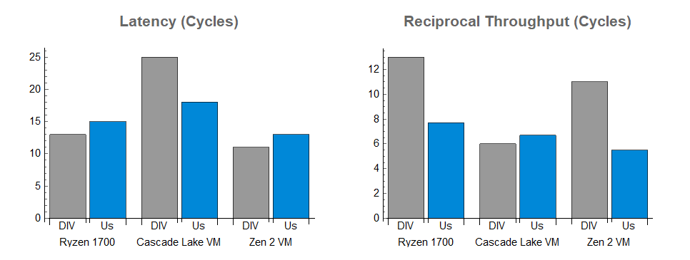
And it does not benefit at all from hardware acceleration. We see slightly better latency for division alone and better throughput on the Intel chips, and much better throughput on Zen 1 and Zen 2. That is not to say that this is a pure win compared to the DIV instruction on those machines, since we are spending extra micro-ops and crowding the other parts of the CPU, but we get some nice results and we have an algorithm that prepares us for a vectorized implementation, where we can get significantly better throughput.
What we Know about Intel and AMD's Solution
The x86 DIV instruction has an impedance mismatch with how it is usually used: the DIV instruction accepts
a numerator that is twice the width of the denominator, and produces a division result and a remainder. Usually,
when you compute a division result with DIV, you have a size_t (or unsigned char) that you want to divide by
another size_t (or unsigned char). As a result, if you want a 64-bit denominator, the x86 DIV instruction
forces you to accept a 128-bit numerator spread between two registers. Similarly, for an 8-bit division, the DIV
instruction has a 16-bit numerator. As such, if you only want the quotient (and not the remainder), or if you want
a numerator that is the same width as the denominator, you don't get the instruction you want.
This kind of abstraction mismatch is important to watch for in performance work: the wrong abstraction can be
incredibly expensive, and aligning abstractions with the problem you want to solve is often the main consideration
when improving the speed of a comptuer system. For today's software, DIV is the wrong abstraction, but since
it is part of the instruction set, we are stuck with it.
Internal Details of DIV
Computer division generally uses iterative approximation algorithms based on an initial guess. However, effective use of these methods requires that you have a decent initial guess: in each iteration these methods square their error, doubling the number of correct bits in the guess, but that isn't very efficient when you start with only one correct bit. As a result, most CPUs have a unit that computes an initial guess.
We have some insight into how Intel and AMD do this - the RCPPS and RCPSS instructions are a
hardware-accelerated reciprocal calculation
function with a guarantee that they are within $1.5 * 2^{-12}$ of the correct reciprocal. Intel recently
released the VRCP14SD/PD instructions in AVX-512, which gives an approximation within $2^{-14}$ (and they
had VRCP28PD, but only on the Xeon Phi). Both RCPSS and VRCPSS are pretty efficient: they perform
similarly to the MUL instruciton.
Intel has released some code to simulate the VRCP14SD instruction: it uses a piecewise linear function to
approximate the reciprocal of the fractional part of the floating-point number, and directly computes the
power of 2 for the reciprocal.
Using the clues we have, we can guess that for integer division, Intel and AMD probably use something like following algorithm:
- Prepare the denominator for a guess by left-justifying it (making it similar to a floating-point number)
- Use the hardware behind
RCPSSorVRCP14SDto get within a tight bound of the answer - Round the denominator or go through one iteration of the refinement algorithm chosen
- Multiply by the numerator and then shift to get the final division result
- Multiply the division result by the denominator and subtract from the numerator to get the modulus (perhaps using a fused-multiply-add instruction of some kind)
And this is all done by a small state machine inside the division acceleration unit, although it probably used to be done with some assistance from microcode in the Haswell and Skylake generations of Intel CPUs.
Function Estimation
It is tempting to use lookup tables of magic numbers, and that is certainly an approach that will microbenchmark well, but in practice, lookup table algorithms tend to perform poorly: one cache miss costs you tens or hundreds of clock cycles. Intel and AMD can use lookup tables without this problem, but we don't have that luxury.
As a first step to DIYing it, let's look at two numerical techniques for generating polynomial approximations: Chebyshev Approximations and the Remez Exchange algorithm. They deserve their own blog post, which is on my list, but here is a very quick overview.
Constraining the Domain
Approximation algortihms work best when we are approximating over a small domain. For division, the domain can be $0.5 < D \leq 1$, meaning that we can constrain $\frac{1}{D}$ pretty tightly as well: $1 \leq \frac{1}{D} < 2$. We will do the other part of the division by bit shifting, since bit shifts are fast and allow us to divide by any power of 2. In order to compute an 8-bit DIV, we would like to estimate the reciprocal of $\frac{1}{D}$ such that we are overestimating, but never by more than $2^{-8}$. We can then multiply this reciprocal by the numerator and shift, and we get a division.
Chebyshev Approximation
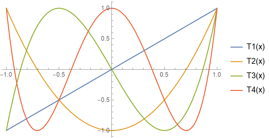
Chebyshev approximation is a method for generating a polynomial approximation of a function within a window. Most people have heard of using a Taylor series to do this, but a Chebyshev approximation produces a result that is literally an order of magnitude better than a Taylor series. Instead of approximating a function as a series of derivatives, we approximate the function as a sum of Chebyshev polynomials. The Chebyshev polynomials are special because they are level: The nth Chebyshev polynomial oscillates between +1 and -1 within the interval [-1, 1] and crosses 0 n times. If you are familiar with Fourier series decomposition, Chebyshev approximation uses a similar process, but with the Chebyshev polynomials instead of sines and cosines (for the mathematically inclined, the Chebyshev polynomials are an orthogonal basis). The first 4 Chebyshev polynomials look like:
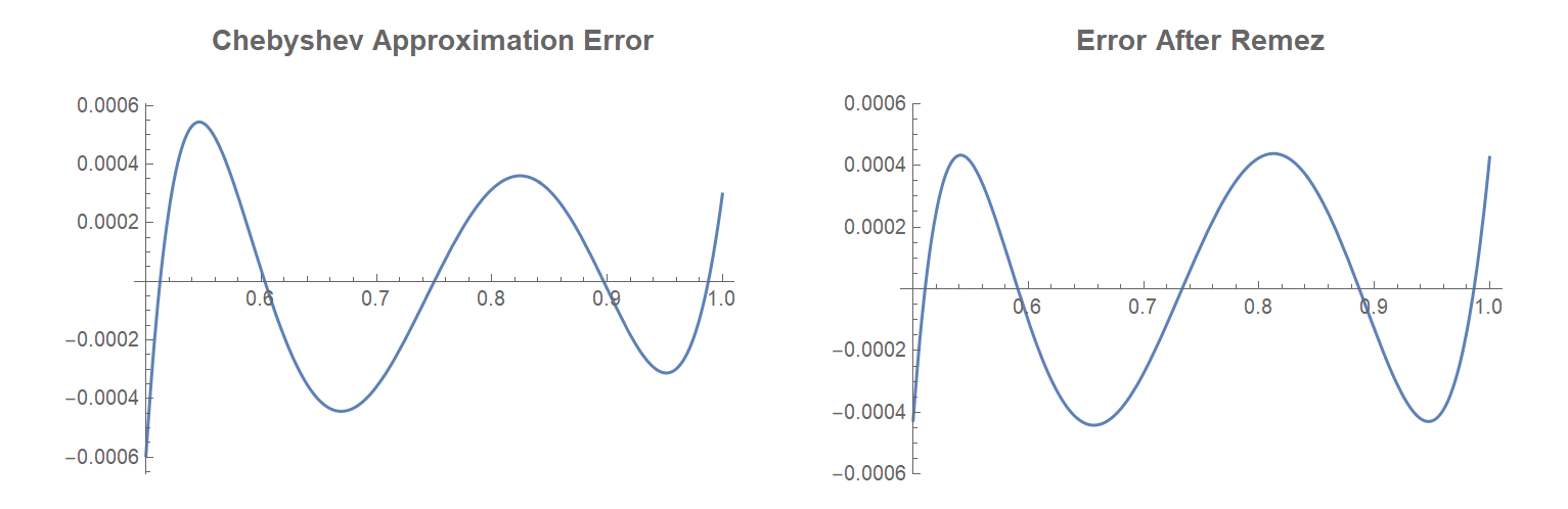
When we do a Chebyshev approximation, we get a much more accurate approximation than a Taylor series:
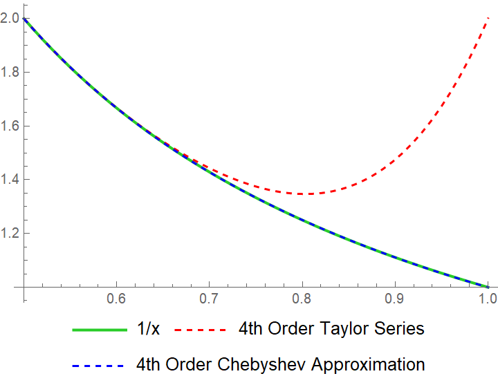
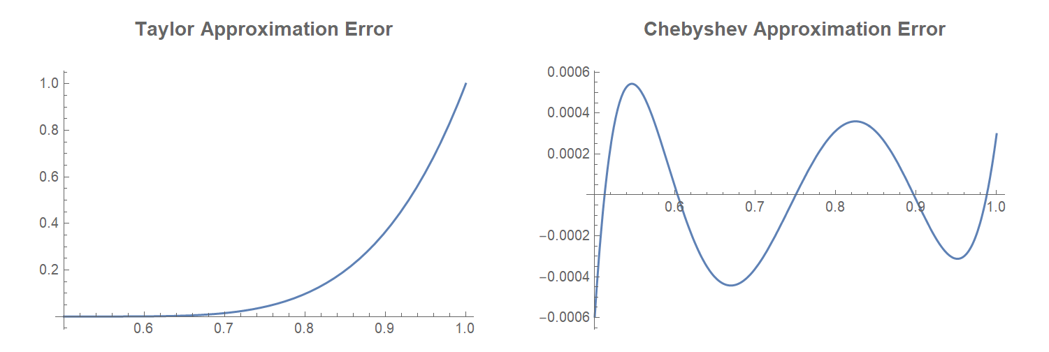
The Chebyshev approximation is almost exactly the same as the function! Instead of error increasing over the input like a Taylor series, the error of a Chebyshev approximation oscillates and the error stays near 0:
The Remez Algorithm
The Remez Exchange algorithm allows you to refine an existing Chebyshev approximation, improving its maximum error by a little bit. Looking at the error of the Chebyshev approximation from above, the absolute value of the peaks decreases as x increases. The Remez algorithm adjusts the approximation to equalize the error over the domain. Since we are trying to minimize the maximum error, this helps the approximation a little bit. After applying one iteration of the Remez algorithm, the error changes from the figure on the left to the figure on the right:
To compare the two approximations, we get the following approximate formulas from Chebyshev and Remez:
$$ Chebyshev(x) = 7.07107 - 19.6967x + 27.0235x^2 - 18.2694x^3 + 4.87184x^4 $$
$$ Remez(x) = 7.15723 - 20.1811x + 28.024x^2 - 19.17x^3 + 5.17028x^4 $$
Improving our Approximation
We want to do two things to improve our approximation to make it useful: (1) we want it to compute faster, and (2) we want it to never underestimate so we can round by truncation (round down). If we shift up the Remez formula a bit, we get something that solves the second criterion:
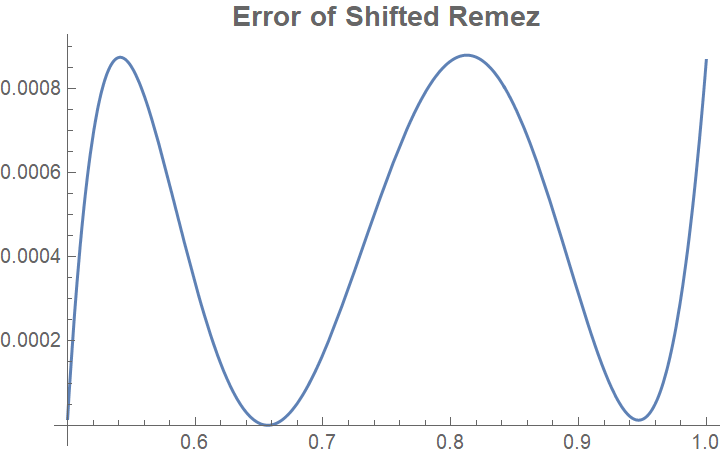
$$ RemezShifted(x) = 5.17028 (1.96866 - 2.6834x + x^2)(0.703212 - 1.02432x + x^2) $$
But not the first. To compute this, we still need 5 multiplication instructions:
- We have to produce $x^2$
- We have to multiply the linear terms in each of the sets of parentheses
- We have to multiply the two parts together
- We need to multiply the whole thing by 5.17028
Eliminating Multiplications
Not all multiplications are equal. Multiplying by 5 is much easier than multiplying by 5.17028. This is because
multiplying a number by 5 is equivalent to multiplying it by 4 (shifting left by 2) and then adding the result to
itself. If you want to multiply by a register by 5 on an x86 machine, you can do it without a MUL instruction:
LEA $result_reg, [$input_reg + $input_reg * 4] performs this calculation. The LEA instruction is
one of the most effective mathematical instructions in the x86 instruction set: it allows you to do several types of
addition and multiply by 2, 3, 4, 5, 8, or 9 in one instruction.
Intel CPUs have a set of units that accelerate array indexing which allow you to compute an address for an array
element. The accelerators compute base + constant + index * size while loading or storing to memory, with size
restricted to a word length (1, 2, 4, or 8 on a 64-bit machine). Instead of loading from memory, LEA directly
gives us the result of the array indexing calculation. This allows us to do simple multiplication, 3-operand addition,
and other similar functions in one instruction (although 3-operand LEAs tend to carry a performance penalty compared
to 2-operand LEA instructions).
The coefficients of the formula we derived with Remez are pretty close to some coefficients that allow us to
use bit shifts and LEAs: $5 \approx 5.17028$, $2.6834 \approx 2.6875$, and $1.02432 \approx 1.03125$.
$$ 1.03125 x = x + (x \gg 5) $$
$$ 2.6875 x = 3 x - 5 (x \gg 4) $$
That gives us the following function:
$$ ApproxRecip(x) = 5(c_1 - 2.6875x + x^2)(c_2 - 1.03125x + x^2) $$
That gives us both coefficients using two SHR instructions, two LEA instructions, one ADD (which
could also be an LEA), and one SUB. Our overall computation now only has two MUL instructions:
one to compute $x^2$ and one to multiply the results from the parentheses. The final multiplication by 5
is another LEA instruction instead of a MUL.
We can use a minimax algorithm to determine $c_1 = 1.97955322265625$ and $c_2 = 0.717529296875$. Needless to say, the function we get is no longer optimal. The error (comparing to $1/x$) looks like this:
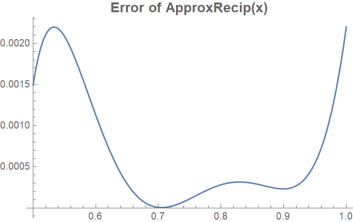
This is not anywhere near as good as our shifted Remez approximation, but it is still good enough: the maximum of the error is a little over $0.0022$, which means we get within 8.8 bits of the correct result of the division. That's close enough for an 8-bit divison! Since we overestimate, we can just truncate to 8 bits, rounding down, and we will get the correct result.
Mapping to Code
Mapping this algorithm to code is going to require a healthy dose of fixed-point arithmetic. We have
talked a lot about numbers between 0.5 and 1, but in order to map this to efficient code, we are not
going to use floating point. Instead, we will use fixed-point: we will treat a certain number of bits
of an integer as "behind the decimal point" and the rest as "in front of the decimal point." At first,
we wil be using 16 bits behind the decimal point, and then later 32 bits. We will refer to them as m.n
numbers, with m bits ahead of the decimal place, and n bits behind. Since we are working on a 64-bit
machine, we are using 48.16 and 32.32 numbers.
Adding fixed-point numbers works like integer addition as long as each fixed-point number has the same
order of magnitude. If not, the numbers have to be shifted to be aligned: when you add a 32.32 number
to a 48.16 number, one needs to be shifted by 16 bits to align it with the other.
Multiplying fixed-point numbers is a bit wierder. When you multiply two 32 bit integers, you get a
result that fits in 64 bits. Often, we discard the top 32 bits of that result to truncate the result
to the same size as the inputs. With fixed-point m.n numbers, you add the number of bits before and
after the decimal place: when you multiply a 48.16 number with a 32.32 number, the result is an 80.48
number, and must be shifted and trucated to select the bits you want. We are going to try to avoid
any shifting if we can, and just use the bottom 64 bits of the result so we can use a single MUL
instruction for multiplication.
One final caveat: for these algorithms, we will be ignoring division by 0 for now. Division by 0 can be handled slowly (it is for the DIV instruction - Intel throws an interrupt) as long as it doesn't impact other results. Thankfully, we have a tool to handle this: branches and the branch predictor. Around each of these blocks of code, we can place a wrapper that checks for division by 0 and gives a specific result (or throws an exception) if you have a division by 0. Thanks to branch prediction, this branch will be free if we are not frequently dividing by 0, and if we are dividing by 0 frequently, it will be a lot better on average than the exception!
Doing it in C
I attempted to write this in C for microbenchmarks, fully expecting the compiler to produce a result that was as good (in a standalone context) as handwritten assembly. Here is the C code:
 1#include <stdint.h>
 2#include <immintrin.h>
 3
 4// Constants computed with minimax
 5static const int C1 = 0x1fac5;
 6static const int C2 = 0xb7b0;
 7
 8int64_t approx_recip16(int64_t divisor) {
 9    // Square the divisor, shifting to get a 48.16 fixed point solution
10    int64_t div_squared = (divisor * divisor) >> 16;
11
12    // Compute the factors of the approximation
13    int64_t f1 = C1 - 3 * divisor + 5 * (divisor >> 4);
14    int64_t f2 = C2 - divisor - (divisor >> 5);
15    f1 += div_squared;
16    f2 += div_squared;
17
18    // Combine the factors and multiply by 5, giving a 32.32 result
19    int64_t combined = f1 * f2;
20    return 5 * combined;
21}
22
23uint8_t div8(uint8_t num, uint8_t div) {
24    // Map to 48.16 fixed-point
25    int64_t divisor_extended = div;
26    uint16_t shift = __lzcnt16(divisor_extended);
27
28    // Shift out the bits of the extended divisor in front of the decimal
29    divisor_extended = divisor_extended << shift;
30
31    // Compute the reciprocal
32    int64_t reciprocal = approx_recip16(divisor_extended);
33
34    // Multiply the reciprocal by the numerator to get a preliminary result
35    // in 32.32 fixed-point
36    int64_t result = num * reciprocal;
37
38    // Shift the result down to an integer and finish the division by dividing
39    // by the appropriate power of 2
40    uint32_t result_shift = 48 - shift;
41    return result >> result_shift;
42}
For a remainder calculation, we just have to do a multiplication and subtraction afterwards.
Hand-tuned Assembly
Since we are racing against hardware and we have a simple function, we want to give ourselves every advantage we can. Let's see how we do with handwritten assembly:
 1# Divide 8-bit numbers assuming use of the System-V ABI
 2# Arguments:
 3#   - RDI = numerator (already 0-extended)
 4#   - RSI = denominator (already 0-extended)
 5# Return value:
 6#   - RAX = division result
 7# Clobbers:
 8#   RCX, RDX, R8, R9, R10, flags
 9
10.text
11div8:
12    # Count leading zeroes of the denominator, preparing for fixed point
13    lzcnt cx, si
14
15    # Put denominator inside [0.5, 1) as a 48.16 number, creating 2 copies
16    # We do two of these instead of using a MOV to improve latency
17    shlx rdx, rsi, rcx
18    shlx r8, rsi, rcx
19
20    # Square one of the copies
21    imul r8, r8
22
23    # Make denominator * 3 to begin the first parenthetical factor
24    lea r10d, [rdx + rdx * 2]
25
26    # Begin producing negative of the second factor by subtracting
27    # C2 from the denominator
28    lea eax, [rdx - 0xb7b0]
29
30    # Copy the denominator
31    mov r9d, edx
32
33    # Negate denominator * 3
34    neg r10d
35
36    # Shift our copies of the denominator
37    shr edx, 4
38    shr r9d, 5
39
40    # Compute 5 * (denominator >> 4) in EDX
41    lea edx, [rdx + rdx * 4]
42
43    # Add C1 to the first factor
44    add r10d, 0x1fac5
45
46    # Make denominator + (denominator >> 5) - C2
47    add eax, r9d
48
49    # Make C1 - 3 * denominator + 5 * (denominator >> 4)
50    add edx, r10d
51
52    # Shift denominator^2 right by 16, going from 32.32 to 48.16, to
53    # prepare for addition to a 48.16 number
54    shr r8d, 16
55
56    # Add the square to each factor, since one is negative we subtract
57    add edx, r8d
58    sub r8d, eax
59
60    # Multiply the factors and then multiply by 5
61    # After this step, we have a 32.32 approximate reciprocal
62    imul rdx, r8
63    lea rax, [rdx + rdx * 4]
64
65    # Multiply the numerator by the approximate reciprocal to get a divisor
66    imul rax, rdi
67
68    # Shift out bits to divide by the remaining powers of 2 and
69    # undo the shift we did to put the denominator inside [0.5, 1)
70    neg ecx
71    add ecx, 48
72    shrx rax, rax, rcx
A remainder calculation is also a matter of a straightforward multiplication and subtraction after the
division, which amounts to an IMUL and a SUB.
Comparison between C and Assembly
Using godbolt.org to inspect the assembled result of the C, a few comparisons come up:
- Clang did significantly better than gcc. With code that is aritmetic-heavy, this is not surprising.
- C compilers (both gcc and clang) used fewer registers than my handwritten solution.
- The best compiled solution (
clang -O3 -march=haswell) involved 25 micro-ops issued, but since 3 of them wereMOVinstructions that copy one register to another, most machines will only have to retire 22 micro-ops due toMOVelision. - Presumably as a result of register allocation, the C had worse throughput and latency.
- Architecture specializations don't appear to change the compiler output significantly.
- Computing the negative of the second factor and using an additional
SHRXinstruction instead of aMOVwas important for latency in the assembly implementation.
Outside of a microbenchmark and in real software, the compiler probably wins due to the register allocation and the reduction in number of retired micro-ops. However, if I were considering a microcoded division implementation for a new CPU, I would likely prefer to spend registers in exchange for speed: a modern x86 CPU has an abundance of registers available to microcode programs (Skylake has 180 integer registers), but only exposes 16 of them at a time to software.
Working with Non-x86 Machines
On a non-x86 machine, you can do something very similar: ARM allows similar instructions to Intel's
LEA instruction with its barrel-shifted operands. RISC-V with the Bitmanip instruction sets is similar.
However, without the bitmanip extension, we don't get the LEA trick, so RISC-V needs several more instructions
for multiplication by 5 and 3. Several of the choices of bit widths in this algorithm are based on which
x86 instructions are the fastest: an ARM or RISC-V solution would need similar care.
Embedded systems these days often have a single-cycle multiplier. In systems like that, the MUL
elimination steps we took are useless: you can do something that is a lot simpler. Using a formula
similar to the $RemezShifted(x)$ formula, you could likely get great division performance on an embedded
system.
On narrower machines, you can do the same calculation with some bit shifting or some implied bits to get similar results without using 64 bit words. You need at least a 16 bit word to do this algorithm, though: with 8 bit words you lose too much precision to quantization. For a vectorized version, we will be using 16-bit words.
Measurements
In order to produce the data tables above, I used llvm-mca to determine the reciprocal throughput of each
solution, and computed latency by hand. The latency difference between Intel and AMD comes down to the lzcnt
instruction: it takes 3 cycles on Intel and 1 cycle on AMD. The assembly code I have proposed here is fairly
portable and has similar characteristics between AMD and Intel cores.
Benchmarks
To verify the theoretical numbers, I ran a few benchmarks using Agner Fog's
PMCTest program on several machines, including some control
benchmarks on DIV.
Here is the control benchmark for DIV:
| Machine | DIV Latency | DIV Recip Throughput |
|---|---|---|
| AMD Ryzen 1700 Desktop | 13 | 13 |
| Intel Cascade Lake (DigitalOcean VM) | 25 | 6 |
| AMD Zen 2 (DigitalOcean VM) | 11 | 11 |
These are the same as the measurements from uops.info. And the results for our division function are:
| Machine | Our Latency | Our Recip Throughput | Our Micro-Ops |
|---|---|---|---|
| AMD Ryzen 1700 Desktop | 15 (+15%) | 7.7 (-40%) | 26.5 |
| Intel Cascade Lake (DigitalOcean VM) | 18 (-28%) | 6.7 (+12%) | 23 |
| AMD Zen 2 (DigitalOcean VM) | 13 (+18%) | 5.5 (-50%) | 23 |
Our benchmark numbers line up with our estimates, and suggest that we have produced something that is in line with the performance of a hardware-accelerated division function. We have ~40% better throughput on AMD Zen 1/2 machines than DIV, with a minor latency penalty. Compared to a recent Intel machine, we have 28% better latency with a 12% throughput penalty.
Once again, in graphical form, here is the comparison between DIV and our function (lower is better on both charts):
Conclusions
It looks like you can produce a CPU with microcoded division that gets close in performance to a CPU with a hardware accelerated unit. That is not to say that Intel or AMD should get rid of their division accelerators: they are comparatively small and the new ones offer better performance than this algorithm. However, you can get very similar performance to the older accelerators with pure software. If you are producing a smaller RISC-V core, though, an algorithm like this looks like it's an option rather than adding a division accelerator. Additionally, it may benefit applications that do a lot of division on Skylake and older CPUs to use this approach rather than dividing with DIV.
For server-class CPUs, the real power of this kind of formula is not in scalar division, but vector division, where hardware acceleration is a lot more expensive. The algorithm will look slightly different: we will probably want to use a 16-bit word length rather than a 64-bit word length.
We also have another loose end: wider divisions. 64 bit division is a lot more useful than 8 bit division, and some machines have very long computation times for 64 bit DIVs (Haswell and Skylake in particular). If we can improve 64 bit division, there may be some places where we can race hardware there too.