The Most Useful Statistical Test You Didn't Learn in School
In performance work, you will often find many distributions that are weirdly shaped: fat-tailed distributions, distributions with a hard lower bound at a non-zero number, and distributions that are just plain odd. Particularly when you look at latency distributions, it is extremely common for the 99th percentile to be a lot further from the mean than the 1st percentile. These sorts of asymmetric fat-tailed distributions come with the business.
Often times, when performance engineers need to be scientific about their work, they will take samples of these distributions, and put them into into a $t$-test to get a $p$-value for the significance of their improvements. That is what you learned in a basic statistics or lab science class, so why not? Unfortunately, the world of computers is more complicated than the beer quality experiments for which the $t$-test was invented, and violates one of its core assumptions: that the sample means are normally distributed. When you have a lot of samples, this can hold, but it often doesn't.
Alternatively, engineers may run several trials of thousands of samples and then use $t$-tests on the descriptive statistics produced by those trials. While this is statistically valid, you may need to expend a lot of resources to run those trials, and the required quantity of tests can limit what information you can test.
Instead, when comparing two samples that are very oddly distributed, my preferred test is the Kolmogorov-Smirnov test. It is a fairly simple statistical test that can be used to compare any two samples (or a sample with a distribution), and directly answers the question of whether the two samples could have come from the same distribution without making any other assumptions.
The Kolmogorov-Smirnov Test
The Kolmogorov-Smirnov test is simple to execute. Consider two samples, $A$, and $B$ with sizes $m$ and $n$:
- Compute the cumulative distribution function (CDF) of each of the samples. For a sample, the CDF is defined as the fraction of the sample that is less than or equal to $x$ for any given $x$. For a continuous distribution, the CDF is the probability that a random value drawn from that distribution is less than or equal to $X$.
- Find the maximum distance between the CDFs, and call it $D$.
In math terms:
$$ D = \max_x \left| CDF_A(x) - CDF_B(x) \right| $$
- Reject the null hypothesis at the $\alpha$ level if the following inequality holds:
$$ D > \sqrt{-\ln\left( \frac{\alpha}{2} \right) \cdot \frac{1 + \frac{n}{m}}{2n}} $$
Alternatively, you can re-arrange this equation to determine a $p$-value for a given $D$:
$$ p = 2 \exp \left[ -D^2 \frac{2n}{1 + \frac{n}{m}} \right] $$
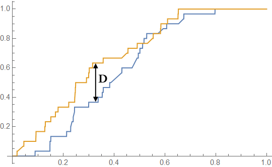
In the example we have above, each of the two samples has 30 points. $D = 0.267$, and the critical value of $D$ at the $0.05$ level is $0.35$. The null hypothesis would not be rejected ($p = 0.24$).
Here is another example, with two samples of 30 points, where the null hypothesis is rejected:
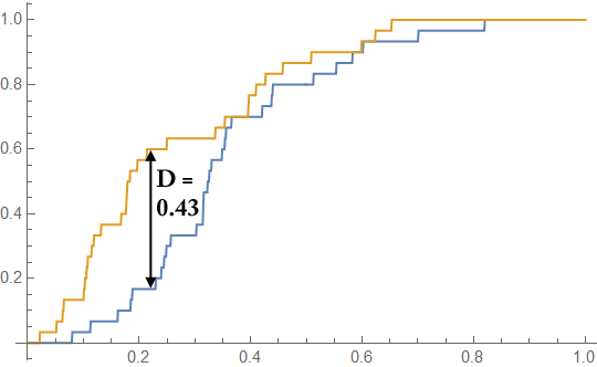
In this case, $D = 0.43$, and $D_{crit, 0.05} = 0.35$. Therefore, with $p = 0.00715$, the null hypothesis is rejected, and the Kolmogorov-Smirnov test concludes that the samples are drawn from different distributions. That is a good thing, because they are drawn from different distributions! In both cases, the yellow sample was drawn from a beta distribution with $\alpha = 2$ and $\beta = 4$, while the blue sample was drawn from a beta distribution with $\alpha = 2$ and $\beta = 5$.
By the way, there is a way to do a multivariate Kolmogorov-Smirnov test, but I have never done one. The algorithms were developed fairly recently, one in 1997 for a sample and a distribution, and a two-sample one in 2004. I would suggest a different test for a multivariate statistical test.
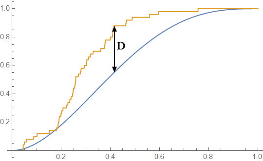
Testing Against a Known Distribution
The other use of the Kolmogorov-Smirnov test is to compare data from an experiment to an expected distribution. In this case, the critical value and $p$-value calculation is given by taking the limit as $m \rightarrow \infty$:
$$ D_{crit} = \lim_{m \rightarrow \infty} \left( \sqrt{-\ln\left( \frac{\alpha}{2} \right) \cdot \frac{1 + \frac{n}{m}}{2n}} \right) = \sqrt{-\frac{1}{2n} \ln\left( \frac{\alpha}{2} \right)} $$
The calculation to find $D$ is the same as before: we look for the point of maximum difference between the two distributions.
So we are now testing for:
$$ \max_x \left| CDF_A(x) - CDF_B(x) \right| > \sqrt{-\frac{1}{2n} \ln\left( \frac{\alpha}{2} \right)} $$
Where $b$ is the size of the dataset being tested, and $\alpha$ is the desired $p$-value. Similarly, the $p$-value calculation for the dataset becomes:
$$ p = 2 e^{-2nD^2} $$
This can be useful as a test of normality or a test of the goodness of fit of a regression. It is also sometimes used for testing random number generators against uniform distributions, and checking for financial and election fraud using Benford's Law.
As an Algorithm
SciPy, the Excel statistics package, R, and mathematical computing packages have pre-written algorithms for Kolmogorov-Smirnov tests. However, it is a pretty easy algorithm to implement. Because of the monotonic nature of CDFs, the maximum will occur at one of the "steps" of one of the CDFs, which happen at the points in each respective set. Thus, we only have to test a very limited number of points to be the possible maximum instead of doing any real math. Here is the two-sample test in (unoptimized) C++:
 1#include <cmath>
 2#include <set>
 3
 4// Kolmogorov-Smirnov test of two ordered sets of doubles
 5double two_sample_ks (const std::set<double>& set_a,
 6                      const std::set<double>& set_b) {
 7    // Doubles of set size and CDFs
 8    double n = set_a.size();
 9    double m = set_b.size();
10    double cdf_a = 0.0;
11    double cdf_b = 0.0;
12
13    // Track the maximum delta between the CDFs
14    double max_delta = 0.00;
15
16    // Iterators through the sets
17    auto walk_a = set_a.begin();
18    auto walk_b = set_b.begin();
19
20    // Walk across the X axis tracking the delta between the CDFs of A and B
21    // The only relevant points to check are places where the CDF changes
22    while (walk_a != set_a.end() && walk_b != set_b.end()) {
23        // Compute the CDFs and the delta between them, tracking the maximum
24        double delta = std::abs(cdf_a - cdf_b);
25        if (delta > max_delta) max_delta = delta;
26
27        // Move to the next relevant position on the X axis and update the CDFs
28        double a_value = *walk_a;
29        if (*walk_a <= *walk_b) {
30            cdf_a += 1.0 / n;
31            ++walk_a;
32        }
33        if (*walk_b <= a_value) {
34            cdf_b += 1.0 / m;
35            ++walk_b;
36        }
37    }
38
39    // Compute the p-value of the test
40    double size_factor = 2.0 * n / (1.0 + n / m);
41    double p_value = 2.0 * std::exp(-max_delta * max_delta * size_factor);
42    return p_value;
43}
If you wanted to do this with a vector or an unordered set, you would have to sort it first. The one-sample test is similarly constrained: the maximum delta will occur either right before or right after a step, so there are again very few points to search to find the maximum delta. Running a Kolmogorov-Smirnov test is just a single pass over the data, and doesn't need any fancy math.
Comparison to $t$-tests
The Kolmogorov-Smirnov test is a non-parametric statistical test: it makes no assumptions about the underlying data. However, like most non-parametric tests, it tends to have higher $p$-values than tests that make assumptions about the underlying data. The strength of the K-S test is that you don't need very many samples to make sure that the test is valid, and you don't need to check the distributions of the data to ensure that the sample means are normal.
As I alluded to above, if you have a very large sample where you can be reasonably sure that sample means are normally distributed, you will probably get a better $p$-value from a $t$-test. Compared to a $t$-test, you can usually run a valid Kolmogorov-Smirnov test with fewer data points, and if the distributions are oddly shaped (eg if they have the same mean, but very different behavior at the tails), the K-S test will often tell you that they are different when a $t$-test might say that the distributions are the same. Remember, a $t$-test tests whether the two samples have different means while a Kolmogorov-Smirnov test determines whether the samples are drawn from different distributions.
Finally, a Kolmogorov-Smirnov test needs at least $O(n \log n)$ time on unsorted data because you need to sort your data to find its CDF. $t$-tests and other similar tests which use descriptive statistics can be computed in $O(n)$ time without sorting the data. However, if you already have sorted data, like database data, you can compute a Kolmogorov-Smirnov test in one pass over the data. A $t$-test similarly needs one pass.
When the $t$-test Doesn't Help
In performance testing, we often see optimizations that help tails of distributions, and keep means relatively unchanged. $t$-tests will reject these effects, while a Kolmogorov-Smirnov test will show an improvement. Here is an example of two datasets with 50 points:
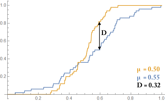
In this case, the two datasets have very similar means: $0.55$ (blue) and $0.50$ (yellow). However, the standard deviations of the distributions are very different: $0.21$ for the blue sample, and $0.11$ for the yellow sample. A $t$-test yields a $p$-value of $0.133$ when comparing these samples, while a Kolmogorov-Smirnov test yields a $p$-value of $0.012$! Visually, these samples are very different, and the Kolmogorov-Smirnov test helps you argue that.
Replacing $t$-Tests with Kolmogorov-Smirnov Tests
Returning to our example of testing a performance improvement, the usual way to solve this problem with $t$-tests is to run a massive number of samples and split the sample pool into several trials. For example, a set of 100,000 runs would be split into 50 "trials" of 2,000 runs. On each trial, you produce descriptive statistics, such as 90th and 99th percentiles, relying on the size of each trial to make sure that the central limit theorem kicks in. These are then compared using $t$-tests, one for the set of 90th percentiles, one for the set of means, etc.
It is a lot easier to use one Kolmogorov-Smirnov test rather than to split your sample artificially so you can use $t$-tests, and you can use it to detect much subtler effects! Alternatively, you can get a similar sensitivity from a Kolmogorov-Smirnov test by running 50 samples that you would get from $t$-testing 50 trials of 2,000 samples each. In both cases, $n = 50$.
When you actually want to compare two means, the $t$-test is the right thing to use. When you want to compare distributions, it is a lot better to use Kolmogorov-Smirnov tests.
Conclusions
The Kolmogorov-Smirnov test is a powerful statistical test that lets you avoid some of the problems of traditional statistical tests. A Kolmogorov-Smirnov test lets you compare an entire distribution against another distribution, so you can detect changes at the tails of a distribution that do not affect the means. It carries no assumptions about the datasets or distributions used. Finally, the Kolmogorov-Smirnov test allows you to accurately scale down these questions to tens of samples. It is a very useful statistical technique to add to your arsenal as a performance engineer or data scientist.